FRAUD DETECTION(1/3)

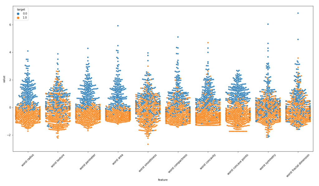
Hello everyone, i am starting out a series of posts which will deal with the very key concepts in data science. I will be writing a series of posts as it is very difficult to accumulate all these important concepts in a single post. The posts will be divided as follows:

  1. Precision and Recall
  2. Synthetic data for imbalance datasets
  3. Credit card fraud detection case study.

So this blog will deal with precision and recall. I will take an example to describe this very important concept. We will be using the credit card fraud detection dataset from kaggle. You can find the dataset in my repo.

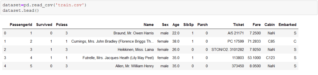
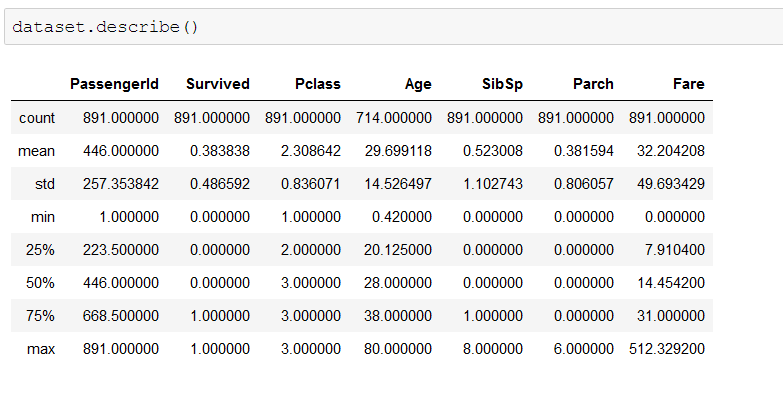
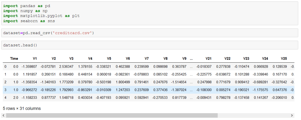
About the dataset
The datasets contains transactions made by credit cards in September 2013 by European cardholders.
This dataset presents transactions that occurred in two days, where we have 492 frauds out of 284,807 transactions. The dataset is highly unbalanced, the positive class (frauds) account for 0.172% of all transactions.Features V1, V2, … V28 are the principal components obtained with PCA, the only features which have not been transformed with PCA are 'Time' and 'Amount'.

Let us start analyzing this dataset and see what insights we can take from it.

I am assuming you are familiar with basic data processing, if not you can see my previous posts. My main aim here is to tell you about Precision and Recall.

Here are some basic steps to start with.

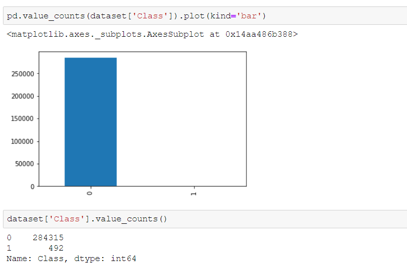
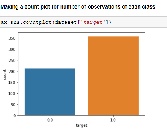
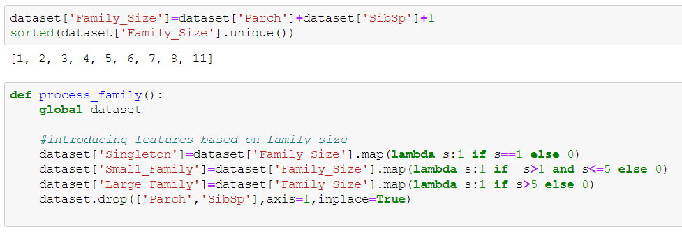
Here we see that our dataset is imbalanced, with very few fraudulent transactions. This type of dataset surely needs to be treated differently but ignoring the fact let us proceed with the mainstream process. We now split the dataset to fit it into logistic regression model.

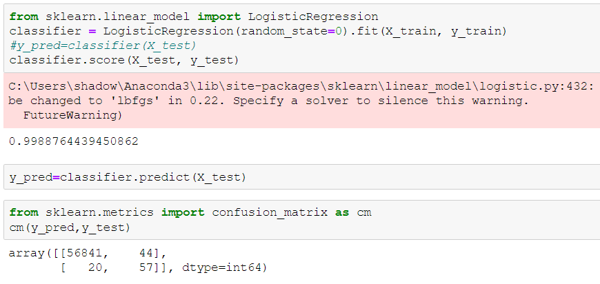
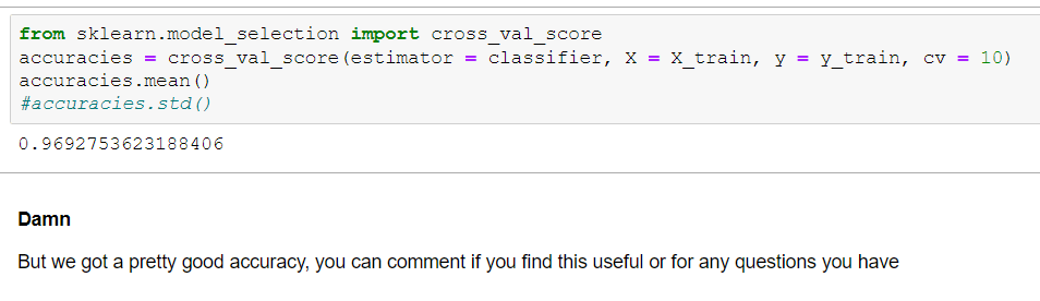
We got an accuracy of 99.8% without any trouble but do you think this is the right approach? Let us now use a dummy classifier. If you’re not aware about dummy classifier you can read about it here. It is basically used for setting a baseline for our future models.

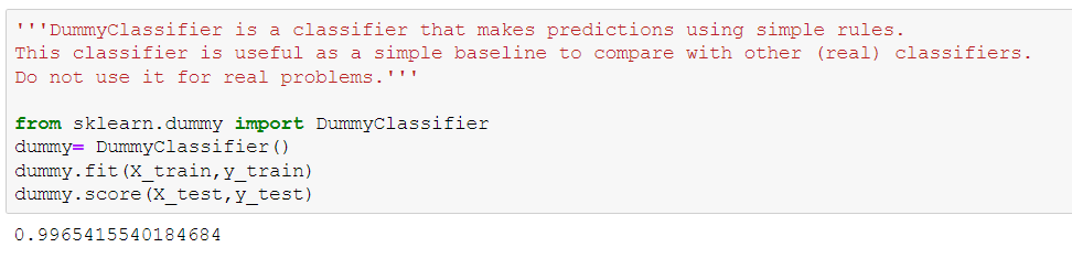
Well now we see a definite problem here. Our model is giving 99.6% accuracy on the dummy classifier model. We sure need to go into a bit deeper to understand what is the anomaly here.

First things first, before we start any data science problem we should always see what the problem is asking us to do. If we are dealing on the larger scale say we have a problem for detecting cancer then our aim should not be to improve the overall accuracy instead we should focus on detecting patients with cancers. For the credit card fraud detection we should focus on detecting most fraudulent accounts. So in short it is always not about overall accuracy. Before moving ahead let us define some basic terminologies which we will use in future.

Confusion Matrix

This is the most basic thing you should be aware about. We will be looking at the basic binary confusion matrix here.

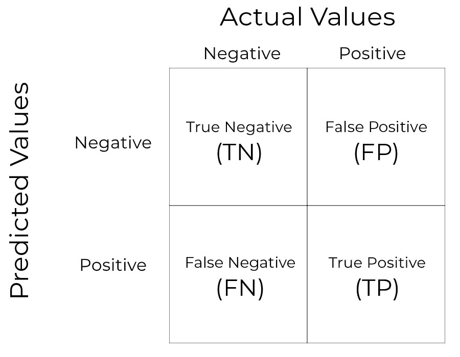
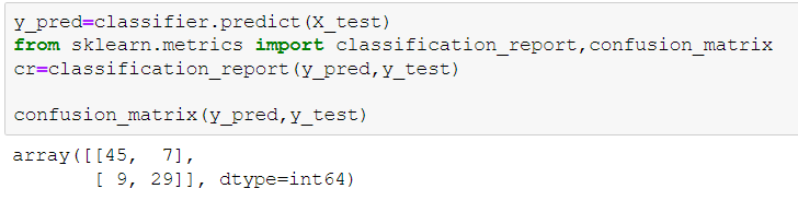
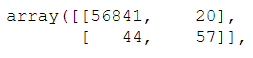
You can compare this with the confusion matrix we obtained for our model. In our problem we are aiming to detect maximum number of true positives(maximum fraudulent customers).

Now we will look at different methods to evaluate our model, all these methods are problem specific i.e you should choose the best one to evaluate your model according to the problem you’re dealing with.

  1. Accuracy- It is defined as total correct predictions divided by the total number of predictions. This evaluation matrix is used when we are not inclined towards predicting positive or negative cases.

Accuracy=(TP+TN)/(TP+TN+FP+FN)

2. Recall- It is defined as out of all the positive classes, how many of them are correctly predicted. For the credit card fraud dataset we need high recall.

Recall= TP/(TP+FN)

3. Precision- Out of all the positive predicted class, how many are actual positive.

Precision=TP/(TP+FP)

An interesting point to note here is that if we are saying our model should have high recall it doesn’t mean that we want our model to have a recall of 1.00 which is also undesirable. Recall of 1.00 will imply that FN=0. For our dataset we want to detect maximum number of fraudulent account but this doesn’t mean that we should label all the accounts as fraudulent ( this would also mean that precision will be 0 as FP is very large). Thus we have to maintain a trade-off between precision and recall. We surely want to maximize both precision and recall (here recall majorly as our dataset demands this).

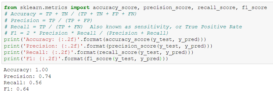
Here we see the value of precision and recall. We surely want to increase our recall. Recall of 0.56 means that our model is classifying only 56% of total fraud instances correctly leaving behind 44%.

I am ending this post here as the main idea was to give an introduction about precision and recall. In the next post we will see how to deal with imbalance dataset.

Breast Cancer Analysis!!!!!!

Hello fellow analyzers!!! Today i will be moving ahead with the series ‘DATA SCIENCE FOR PUPPIES’ and showing my analysis on the breast cancer dataset. You can refer to the code directly as i will be showing very relevant information only, so if you want to get all the analysis i did, you can refer the code.

LINK TO CODE: https://github.com/shadow9909/MyDataScience/tree/master/breast%20cancer

The dataset in available in sklearn.datasets so you don’t need to download it separately. Here is the data description i picked from kaggle but i don’t think you want to go through it. Let us visualize pretty curves.

Attribute Information:

  1. ID number

  2. Diagnosis (M = malignant, B = benign)

3-32) Ten real-valued features are computed for each cell nucleus:

a) radius (mean of distances from center to points on the perimeter)

b) texture (standard deviation of gray-scale values)

c) perimeter

d) area

e) smoothness (local variation in radius lengths)

f) compactness (perimeter^2 / area – 1.0)

g) concavity (severity of concave portions of the contour)

h) concave points (number of concave portions of the contour)

i) symmetry

j) fractal dimension ("coastline approximation" – 1)

Missing attribute values: none

Class distribution: 357 benign, 212 malignant

Let us start analyzing now!!!

Importing all the required libraries, loading the dataset and looking for feature names.

As we have many features it is important to find the best features among them to make our analysis more efficient.

Using correlation matrix for analyzing

What a trippy heatmap it was!! We have to make other visualizations to get more insights of the features.

We will make violin plots and swarm plots here to get a better insight about distribution. Normalizing the dataset and then using pandas melt function for visualization. As the number of features are large we are visualizing them in parts.

We can surely some distributions which are kinda same. Removing these features may/may not affect the performance. But the features with extremely high correlation score surely affects the model. Let us visualize some pairs of feature to obtain their pearson r value.

Features with this high pearsonr value should be removed. I tested the model by both keeping and removing these features. It turns out our model responds well with these features removed.

Here is the list of correlated features. You can check for more such features!!

Now should start the more fun part!!

Note: I have tried many other models and applied parameter tuning to them also. I have showed limited and more relevant things here. You can checkout my notebook for briefer outlook.

Quick dive into titanic dataset

The sinking of the Titanic is one of the most infamous shipwrecks in history.

On April 15, 1912, during her maiden voyage, the widely considered “unsinkable” Titanic sank after colliding with an iceberg. Unfortunately, there weren’t enough lifeboats for everyone onboard, resulting in the death of 1502 out of 2224 passengers and crew.

  1. Analyzing each feature and check whether it is important in our analysis?
  2. What are the most important features to estimate the death?
  3. Generating new feature to improve the accuracy of model?

Data Understanding:Titanic dataset consists data of 891 people . Dataset was investigated before any preprocessing.

Prepare Data: Including data cleaning, filling NAN value, one-hot encoding and MinMax preprocessing. Please refer to Preprocessing for detail.

Data Modeling: Used GridSearch with 5 folds validation to find best parameter for GradientBoostingRegressor. Some other models are trained and compared as well beforehand. Please refer to Training for detail.

Evaluate the Results: Note book of the analysis is on my git repo, you can directly check that out also.

https://github.com/shadow9909/MyDataScience

Let us now dive into the dataset , here I will not be sharing the code directly. You can see the notebook if you want to refer to the code.

Now let us have a sweet look on the dataset and the values.

Checking out the distribution of the values in the numerical columns

Now let us start our column wise analysis

Well we surely saw some serious gender discrimination here.

Now analyzing whether the fare of passengers’ ticket determined their survival.

Splitting embarked class into different columns for analysis

Extracting title from names to check if the model performance will get affected

We got model accuracy of 91.7%

Running tests on test dataset.

No Face Touching

Across the world, government and healthcare authorities are working together to find solutions to combat COVID-19 pandemic and to protect people. As we all know that life after the COVID-19 lock down will not be easy. People will be in a state of trauma and fear. Everyone will be more cautious towards personal hygiene. As research suggests, the virus can only enter our body when infected hands are touched to the face and we all know that it is not possible to wear a mask all the time and we should be aware of the fact that the mask needs to be changed /sanitized after a certain time period.

So we designed a simple yet efficient solution for this. We made two different devices, a wrist band and a neck band, both will enable the buzzer sound if we try to touch our face. This device will activate in a range of 10 to 12cm. It might seem a bit bulky right now because we made this with limited components which were available during lock down. This can be easily reduced if we use more optimized components. We believe that there is no better way to get through this, than by using technology and innovation.

We, in our day to day life are more likely to rub our eyes. As we are going outside it is obvious that we touch things and if it is something which carries the contagious virus then it can further lead to a count in list of corona infected people. Most of the countries are dealing with this issue, these small initiatives can lead to the end of this virus.

We also want to use this device as a tool to make sure that people can, at least get a reminder to stay safe from this virus.

#StaySafe #StopFaceTouching

Recurrent Neural Network

Recurrent Neural Networks are the most advance algorithm that exist in the world of supervised deep learning. As we know neural networks mostly resembles the inner functioning of our brain so it is easy to relate all the things accordingly.

The human brain has got 3 parts: cerebrum , cerebellum and brainstem, which connects the brain to the organs. Then, the cerebrum has 4 lobes

  1. Temporal Lobe: Represent long term memory and is used in Artificial Neural Networks(ANN) in which the weights and bias are to be remembered to make any predictions.
  2. Occipital Lobe: Represent recognition and image processing ,used in Convolution Neural Networks(CNN).
  3. Frontal Lobe: Represent short term memory ,used in Recurrent Neural Network(RNN).
  4. Parietal Lobe: Responsible for sensation, perception and constructing, could be used in future models.

What is Recurrent Neural Network(RNN)?

Recurrent nets are the type of Artificial Neural Networks(ANN) used to recognize patterns in sequences of data. These algorithms take time into account, they have a temporal dimension. They can be used in speech recognition, language modeling, translation, image captioning and stock market prediction.

The main difference which lies between of Artificial Neural Networks (ANN) and Recurrent Neural Network(RNN) is that RNN also uses previous results in addition to current input as their whole input. The decision made by an RNN at time ‘t’ is dependent on the result obtained at ‘t-1‘ . So RNN have two inputs at a particular timestamp, the present input and the recent past and the result which processes to evaluate the correlations between the events separated by events to evaluate further results.

h_t : hidden state at time ‘t’.
W: weights at time ‘t’
x_t: current input
h_t-1: results at time ‘t-1’
U: weights at time ‘t-1’

Visualization of Recurrent Neural Network(RNN)

It would be easy to visualize the RNN if we try to look it transform from ANN. Let us take a simple ANN with 3 input values, 1 hidden layer with 4 nodes and 2 output values.

fig-1

ANN can be converted to RNN by squashing the whole network.

fig-2

It will be easy to visualize if we assume the ANN to be a 3-D structure with nodes to be assumed as ball and connections to be wires. Constructing fig-1 network as described and looked from top gives the view as in fig-2.

fig-3

Simple representation of a network where all the respective layers are vector of values
fig-4

This is an old-school representation of RNN

The neural network in fig-4 shows this hidden layer not only gives an output but also feeds back into itself.

fig-5

Unrolling the network in fig-4 gives the network in fig-5. The network represents flow of data with time and what inputs and values the provides at a particular timestamp

Functioning of RNN

Types of Recurrent Neural Network(RNN)

One to man: This is a network with one input and multiple outputs. This type of network can be used in image captioning. Firstly the image if fed to Convolutional Neural Network (CNN) and then to RNN to make the predictions. CNN gives the features whereas RNN make sense out the sentence predicted.


One to man

Many to one: This type of network have multiple inputs and make a single prediction. This type of network can be used in sentimental analysis.


Many to one

Many to many: This is a network with multiple inputs and multiple outputs. This type of network can be used to generate subtitles. That’s something you can’t do with CNN because you need context about what happened previously to understand what’s happening now, and you need this short-term memory embedded in RNN.

Mant to many

This was the basic intuition of RNN. Hope you found this useful in someway.